October 15th 2017 - John Guibas & Tejpal Virdi
Introduction
Modern generative models, including DCNN’s, GAN’s, and VAE’s, try to produce an entire image at once. However, as we scale the resolution of these images, the memory constraints of our network exponentially meet their limit. As a result, most images produced from generative models today barely meet a size over 500,000 pixels. For a 3-channel image, that’s only ~410x410.
Compositional Pattern-Producing Networks (CPPNs) address this problem (although they are probably not the best for regular image-generation purposes). Instead of generating the entire image at once, CPPNs take an iterative approach to the problem: they generate pixels one by one. These networks take the location of the pixel as input, theoretically allowing for these networks to produce images of any desired resolution given that you input all the locations.
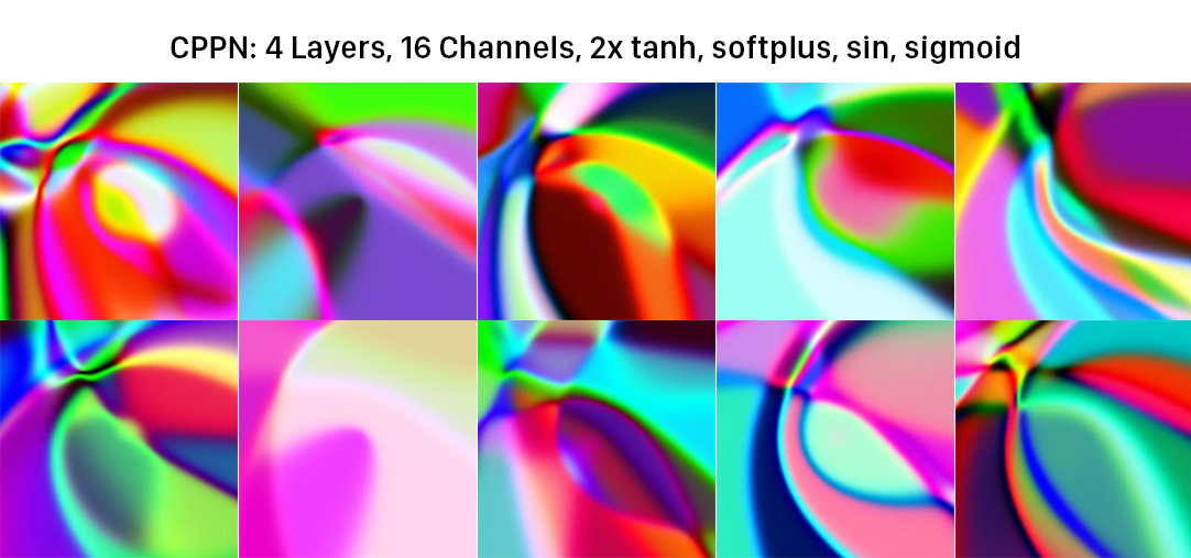
One cool thing about these networks is that even if they are not trained, they produce really interesting patterns that are not just the resemblance of random noise (what you would expect from a random ANN). Here are some examples of images we produced using our CPNN in PyTorch (github):
CPNN Architecture
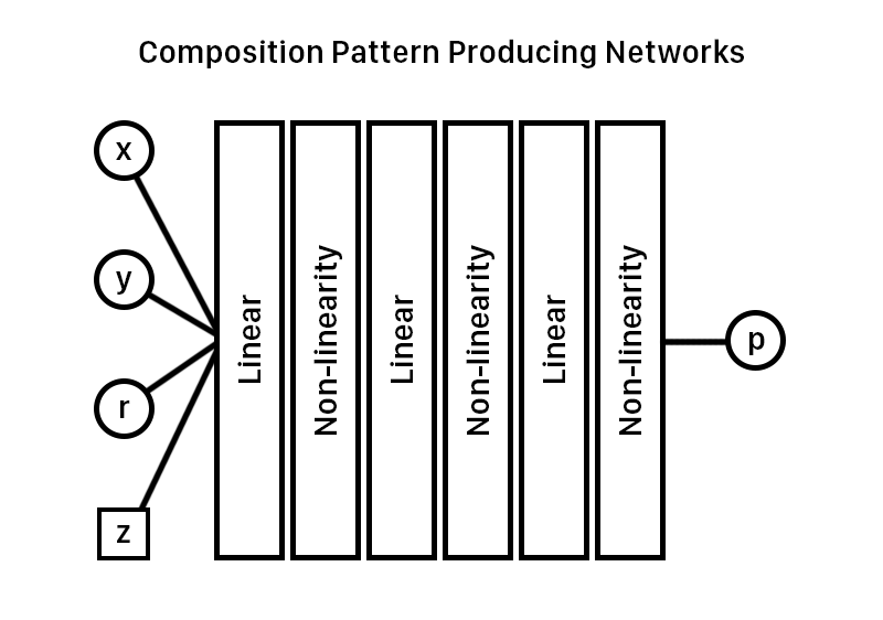
As mentioned above, the CPNN takes in the location as two of its inputs. Another value it takes is the radius of the location, or r= sqrt(x^2 + y^2). This value is essential to the quality of images produced, as it helps the network generate circular patterns without having to curve-fit to such function (highly unlikely without training). The network also takes a latent space vector, which is essentially a series of n elements that are essentially just random variables inputted into the network.
Why do we need such a thing? We really don’t, but it’s nice to have around as by exploring the images in the R dimensions of that vector, we can explore a large amount of images without modifying the weights in the network. In bigger networks, simply modifying one weight won’t be enough compared to changing a value in the latent vector. Also, because our NN is a continuous function, if we adjust the latent vectors position continuously, our output will also be continuous; this leads to cool animations where we can see our network explore the latent space:
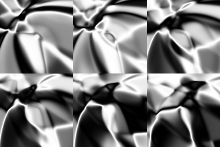
Generated Images
Because our weights are completely random, the non-linearities/activation functions, network depth/size have a big difference in what types are produced by the network. Another interesting fact about these images are that even if I scale the resolution of the image dramatically, overall the image looks the same if I use the same weights. It is important to note that these weights are completely random, and it is quite surprising that they don’t simply produce noise. Anyways, here are a collection of images we produced using a variety of hyperparameters / architectural modifications on our CPPN network:

We can observe how as we increase the amount of channels, the more complex the image becomes. The images more and more start to look the same.

We also experimented with how well the images kept form if I tried to generate the same image at a higher resolution (using the same weights). We can observe how overall the image stays the same and how CPPN’s are resolution invariant.
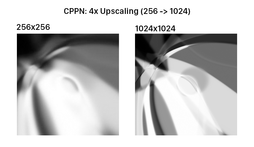
Overall, we can notice that the image has seem to gotten sharper while maintaing the overall strcture.